Nicholas Giordano

As computers are integrated ever more tightly into the educational experience, students are becoming increasing comfortable and proficient with computational methods. Software packages such as Mathematica and Matlab are easy to use, and can be employed for quite sophisticated calculations. This makes it possible to incorporate computational methods into many elementary classes, and thereby explore problems that are not ordinarily accessible. One such topic is realistic projectile motion. The motion of “ideal” projectiles is a fixture in introductory mechanics. By “ideal” we mean that the projectile moves with a constant acceleration, due to the gravitational force. Standard problems include calculations of the range of a batted baseball, and the demonstration that the maximum range occurs when the initial velocity makes an angle of 45° with the horizontal. A typical example might be to calculate the range of a batted baseball. In the major leagues, a baseball may leave the bat with a speed of 110 miles per hour (mph), and in the ideal case this would result in a range of more 800 feet (approximately 250 m). A typical major league home-run rarely travels more than 450 feet, and many are much shorter than this. Moreover, the center field fence in most major league ballpark is generally about 400 feet from home-plate. Hence, it is clear that this calculation greatly overestimates the true range. Even so, many classes (and many textbooks) stop at this point, since the natural next step is to include the force due to air drag.

The difficulty with including the effect of the drag force on such a projectile is that this force is a function of the velocity, and a simple analytic treatment of the trajectory is not possible when the drag is included. A few texts mention the result of Stokes for the drag force, and use this to introduce the notion of a terminal velocity, but the effect of drag on a projectile is rarely discussed. Stokes showed that for an object moving slowly through a fluid, the magnitude of the drag force is

(1)

where ? is the viscosity of the fluid, r is the radius of the object (assumed to be a sphere), and v is its velocity.

With this form for the drag force one can readily calculate the terminal velocity of a sky-diver, etc. However, it turns out that for a real sky-diver this expression for the drag force is completely wrong. The Stokes result applies only for slowly moving objects. Stokes did the calculation so that he could understand the motion of a Foucault pendulum and similar slowly moving things. For nearly all “every day” projectiles, such as baseballs, the Stokes result applies only at velocities below about 1 m/s. At higher velocities

the drag force is given instead by

(2)

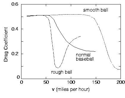
where ? is the density of the fluid (usually air), A is the cross sectional area of the object, and C_D is known as the drag coefficient. As you might guess, the calculation of C_D is quite complex, as it depends on the nature of the air flow (the aerodynamics) around the object. One can give a very simple argument that leads to C_D∼1/2 and this value works surprisingly well for many objects (to within a factor of 2) if the velocity is not too large. Figure 1 shows the behavior of the drag coefficient as a function velocity as measured for a baseball.

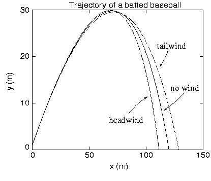
Figure 1. After Ref. 1.

This figure shows the behavior of the drag coefficient for a normal baseball, and also for a rough ball and a smooth ball. Here a “smooth” ball would be one without stitches while a “rough” one would have many more stitches than a regular baseball. While the drag coefficient for all three balls is close to 1/2 at low velocities, it drops at high velocities, and the threshold at which it drops is lowest for a rough ball. The reason for this is the onset of turbulence in the air-flow around the ball. When the flow is turbulent, the air is able to slip past the ball more easily than when the flow is normal (laminar), resulting in a smaller drag coefficient. Note that while the drag coefficient is smaller at high velocities, the drag force is not; F_D continues to increase due to its dependence on v² (see Equation 2).

It is not possible to give an analytic calculation of the trajectory of a baseball with the drag force in Equation 2 (with the drag coefficient in Figure 1) included. However, this trajectory is easily found using a computational approach. When I teach computational physics, I use this as one of the first exercises, since the physics is easily explained (and most students even find it to be interesting!). The trajectory of this realistic projectile is readily computed with a finite difference algorithm, as discussed in Ref. 1. In fact, this problem can be used to introduce and compare different types of algorithms for the numerical solution of differential equations. Some typical results from such a computation are shown in the figure below.

Figure 2.

Figure 2 shows the trajectory of a baseball (the regular ball in Figure 1). Here the ball was given an initial velocity of 110 mph (approximately 50 m/s) at an angle of 35° with respect to the horizontal. The effects of a gentle (10 mph) wind, either at the batter’s back or in his face, are also shown. These results were calculated at the angle that gives the maximum range, which is approximately 35°. Students are quick to recognize that this is a more realistic angle than the value of 45° that yields the maximum range for an ideal projectile. The magnitude of the range found with air drag is also in good accord with observed values.

We believe that there are several morals to be learned from this exercise. First, this is a nice vehicle for introducing computational methods into the classroom. It is an elementary problem, and the computational methods are straightforward, yet this is a problem that can be attacked in no other way. Second, it lets students see that physics can treat the “real” world. They tend to get tired of frictionless inclines, etc.; it is useful for them to see how physics can deal with a realistic situation. Third, this example can be extended in various ways. For example, it can lead into a discussion of the physics of air drag, and similar methods can be used to deal with the motion of a spinning projectile, such as a curve-ball or a golf ball. It can even address the eternal question of why golf balls have dimples (see Ref. 1 for more on this).

(1) Computational Physics, N. Giordano, Prentice-Hall, 1997.

Nicholas Giordano is in the Department of Physics at Purdue University. His research interests include the behavior of metals at nanometer length scales, the acoustics of the piano, and computational physics.